Imaging-transcriptomics
Construct main class of zoom
After preparing the required data, we construct ZOOM_SC, the main object used in zoom class,
using the following code:
>>> from core import ZOOM_SC
>>> zoom_obj = ZOOM_SC(
        adata=adata,
        expression=hcp_expr,
        SBP=SBP,
        SBP_perm=SBP_perm,
        best_comp=None,
        cv=10
    )
Notably, if you only wish to explore the conventional imaging–transcriptomics paradigm and do not
intend to extend to scRNA-seq dataset, you construct a ZOOM object, in which case providing an
additional adata is unnecessary:
>>> from core import ZOOM
>>> zoom_obj = ZOOM(
        expression=hcp_expr,
        SBP=SBP,
        SBP_perm=SBP_perm,
        best_comp=None,
        cv=10
    )
Note
For all analyses on this page, both the ZOOM object and the ZOOM_SC object are equally
applicable. However, if you intend to perform downstream single‑cell analyses, be sure to
construct a ZOOM_SC object and prepare the adata.
Arguments to zoom.core.ZOOM() and zoom.core.ZOOM_SC()
- best_comp int, default None
Optimal number of PLS-R components. If None,
zoomwill determine it via cross-validation.
- cv int, default 10
Number of cross-validation folds.
Partial least squares regression
Partial least squares regression (PLS‑R) model is widely used to associate SBPs with AHBA gene
expression profile. zoom adopts the cross‑validation approach used by Wang, Y. et. al. to determine the optimal component number for
PLS-R model. Further, zoom evaluate how well weighted gene combinations predict SBPs, and
assess whether predictive performance reflects genuine biological underpinnings or spatial
autocorrelation utilizing permutated SBPs. The PLS‑R analysis can be implemented with the
following code and we can print Pearson’s correlation between observed and predicted SBP,
\(Q^2\) (cross-validation \(R^2\)) and \(p_perm\):
>>> zoom_obj.cv_PLSR(
        ncomps=range(1,16),
        repeats_cv=30,
        repeats_pred=101
    )
>>> print(zoom_obj.PLS_r, zoom_obj.PLS_Q2, zoom_obj.PLS_p_perm)
0.8020500907513676  0.6419170826488139  0.001
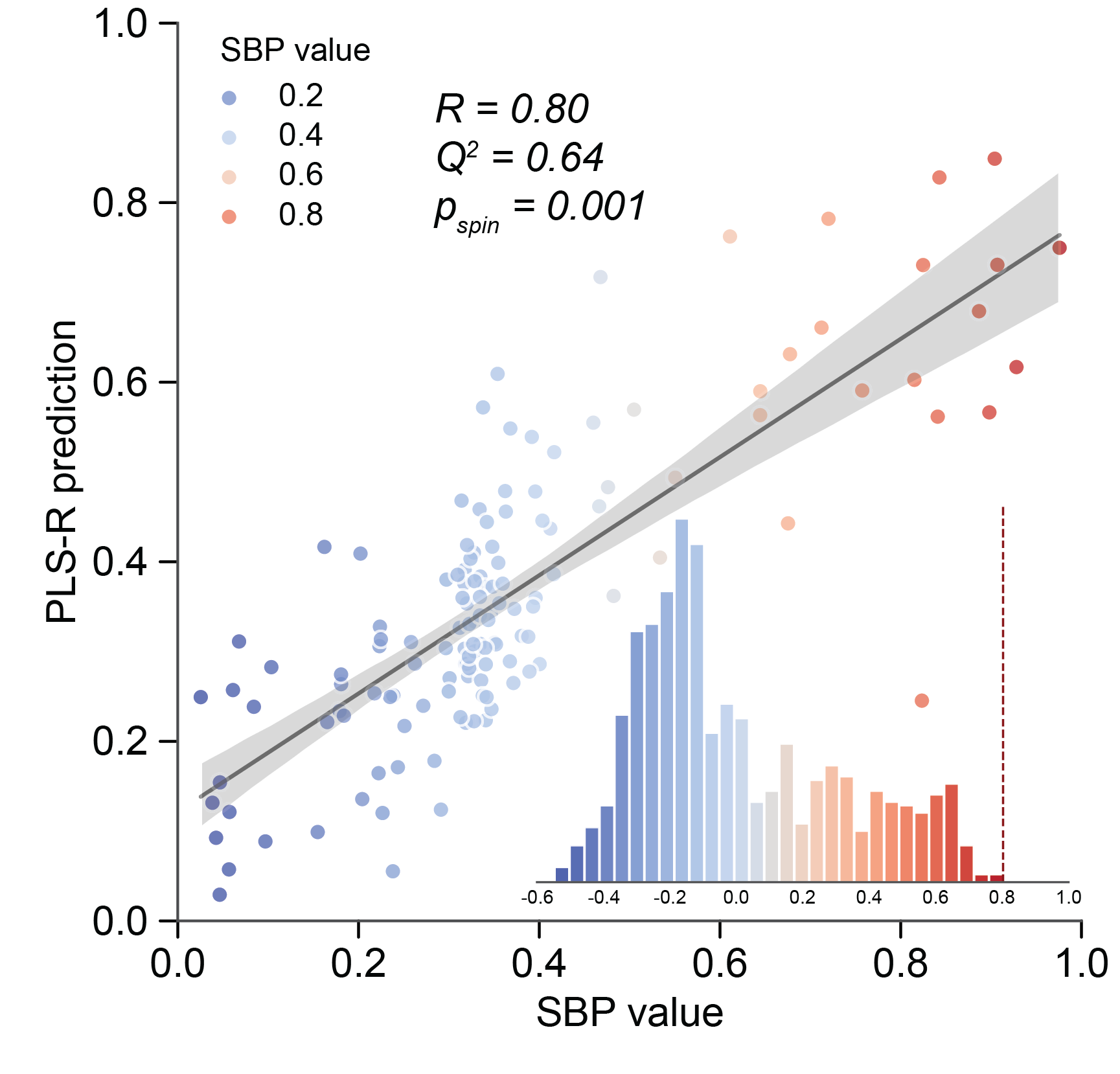
Fig. 6 Dot plot of SBP value and PLS-R prediction, with empirical null distribution of Pearson’s correlation between SBP value and PLS-R predictions trained on permutated SBPs shown on embedded histogram.
Note
Note that the obtained optimal number of component is available as zoom_obj.best_comp. Within
a given range, the PLS‑R model’s predictive performance on the test set typically improves with
increasing component number up to a point (underfitting) and then declines (overfitting). Therefore,
if zoom_obj.best_comp equals 15 in the above procedure, this does not necessarily indicate a
global optimum. You may search over a wider range by re-setting ncomps. Testing more candidate
values increases computation time, which can be mitigated by using a smaller repeats_cv.
Arguments to class method ZOOM_SC.cv_PLSR()
- ncomps {list, numpy.ndarray} optional, default range(1,16)
Optimal component number candidates.
zoomwill pick optimal component number among these candidates.
- repeats_cv int, default 30
How many times should optimal component evaluation be run?
- repeats_pred int, default 101
How many times should model performance evaluation be run? The final performance is defined as the median Pearson’s correlation among
repeats_predtimes repeats.
After running the above class method, the PLS‑R results are stored as the attribute can of ZOOM_SC.
- PLS_r float
Median Pearson’s correlation between predicted SBP value and observed SBP value.
- PLS_Q2 float
Median predictive accuracy of PLS-R model.
- PLS_p_perm float
P-value of spatial permutation test, defined as the proportion of null distribution that exceeded the real model performance.
Gene contribution statistics
Next, we aim to quantify each gene’s contribution in predicting SBPs using the AHBA dataset. zoom
provides three PLS statistics, namely variable importance in PLS prejection (VIP), regression coefficient
(RC), and noemalized PLS1 weight (PLS1). VIP serves as an example here. zoom also simultaneously
evaluates whether gene contributions represent spatial‑autocorrelation‑driven false positives by comparing
to permuted SBPs:
>>> zoom_obj.get_gene_contrib(metric="VIP")
>>> zoom_obj.PLS_report
            Weight  Sign  p_perm
gene
A1BG      0.746265    -1   0.339
A1BG-AS1  1.040469    -1   0.244
AAAS      0.935083    -1   0.145
AAED1     0.790452     1   0.070
...            ...   ...     ...
ZYX       0.625381    -1   0.414
ZZEF1     0.803275    -1   0.240
ZZZ3      0.843117    -1   0.195
[7773 rows x  3 columns]
Here, a positive Sign indicates the gene points in the positive direction of the given SBP, and
a negative Sign indicates the opposite. Weight denotes the gene’s contribution to the PLS‑R prediction,
and p_perm is the gene‑level p‑value from the spatial permutation test. Since VIP is unsigned, the Sign
reported for VIP is taken from RC.
Note
You may notice that the number of genes in zoom_obj.PLS_report (7773) does not match the original
AHBA dataset (7973). This is because when constructing a ZOOM_SC object, zoom automatically
filters the genes in adata and the AHBA dataset, retaining only their intersection.
Arguments to class method ZOOM_SC.get_gene_contrib()
- metric str, default "VIP"
The statistical metric used to quantify gene contribution to PLS-R prediction. Must be one of {“PLS1”, “RC”, “VIP”}. - PLS1: Normalized PLS1 weights estimated through bootstrap strategy, please also specify
n_boot=1000if you use PLS1.
RC: Regression coefficient.
VIP: Variable importance in projection.
Pick optimally sized gene set
Before performing single‑cell scoring, we must verify whether the variables (genes) highlighted by the gene
contribution statistics are biologically meaningful and determine the gene set size for downstream analysis.
To do this, zoom first sorts zoom_obj.PLS_report by p_perm ascending (ties broken by Weight
descending), then selects the top n genes separately from the positively signed genes and negatively
signed genes to form a gene set, constructs an AHBA subset from this gene set to predict the SBP, and finally
assesses predictive accuracy using \(Q^2\). You can quickly do it with following code:
>>> Q2_stats = zoom_obj.test_gene_size(gene_sizes=[30,40,50,75,100,150,200,250,300,400,500])
>>> Q2_stats
                 Q2
gene size
30         0.769825
40         0.822449
50         0.837205
...             ...
300        0.883933
400        0.861235
500        0.857694
[11 rows x  1 columns]
Selecting the top 40 highlighted genes from both directions respectively already yields PLS‑R predictive accuracy far exceeding that obtained using all genes. Further increasing the gene size does not significantly improve predictive accuracy. Thus, 40 genes capture the vast majority of the information needed to describe one direction of the given SBP, and adding more genes primarily introduces noise.
Arguments to class method ZOOM_SC.test_gene_size()
- gene_sizes list
List of candidate gene set sizes.
Spatial permutation-based GSEA
If you wish to further test which biological pathways are more associated with a given SBP, zoom also
provides a spatial permutation–based GSEA. Conventional GSEA permutes the gene ranking to generate a
null distribution, whereas the spatial permutation–based GSEA derives control gene rankings from permuted
SBPs. Here we use the GO: Biological Process(2025) downloaded from enrichR as an example:
Note
Because VIP and RC reflect each gene’s overall contribution across all PLS components, their gene rankings represent weighted combinations of multiple pathways and are therefore unsuitable for simple pathway enrichment under a GSEA framework. We therefore recommend using PLS1 as the gene‑contribution metric for simple pathway analysis, as in the example below. However, for gene sets that inherently combine multiple pathways, such as gene co‑expression modules, using RC or VIP rankings is plausible and recommended since PLS1 always fails to capture meaningful biological underpinnings when the first component does not explain the majority of total variance of given SBP.
>>> from gseapy import read_gmt
>>> BP = read_gmt("/path/to/GO_Biological_Process_2025.gmt")
>>> gsea_res = zoom_obj.GSEA(
        gene_sets=BP,
        min_size=50,
        max_size=500
    )
>>> gsea_res
                                                             ES        NES  p_perm  p_perm_fdr
Term
Cation Binding (GO:0043169)                            -0.59988  -1.537195   0.000       0.000
Protein Serine/Threonine Kinase Activity (GO:0004674)  0.343912   1.380443   0.004       0.216
...                                                         ...        ...     ...         ...
Arguments to class method ZOOM_SC.GSEA()
- gene_sets dict
Gene sets for enrichment analysis, must be organized as {‘Term1’: [Gene1, Gene2,…],…}, or a dict of the above gene sets, with keys indicating the name of dataset.
- min_size int, default 50
Minimum size of target gene set to be included in GSEA analysis
- max_size int, default 500
Maximum size of target gene set to be included in GSEA analysis