Prepare input data

The Allen Human Brain Atlas dataset

Spatial alignment of spatial brain phenotypes (SBPs) with transcriptomic data requires downloading and preprocessing the anatomically comprehensive AHBA dataset. The preprocessing pipeline implemented in zoom, adapted from Dear, R. et al., is optimized for cortical samples. For whole-brain or subcortical analyses, alternative toolkits such as abagen are recommended to enable customized AHBA preprocessing. To improve the accuracy of spatial registration in the AHBA dataset, we recommend using donor-specific parcellation images. zoom also provides an interface for rapid access to these parcellation images. You can prepare parcellated AHBA data into HCP-MMP1.0 atlas with the following Python codes:

>>> import zoom.prepare as pp
>>> atlas_hcp = pp.fetch_atlas(atlas="HCP-MMP")
>>> hcp_expr, hcp_ds = pp.abagen_ctx(
        atlas=atlas_hcp["image"],
        atlas_info=atlas_hcp["info"],
        data_dir="/path/to/ahba/microarray",
        donors_threshold=3,
        gene_stability_threshold=0.5
    )
>>> hcp_expr
           A1BG  A1BG-AS1      AAAS  ...       ZYX     ZZEF1      ZZZ3
label
1      0.234124  0.260771  0.686152  ...  0.839740  0.825577  0.346719
4      0.363618  0.284738  0.681523  ...  0.810666  0.738654  0.357823
5      0.219162  0.217884  0.648171  ...  0.784044  0.761205  0.309604
...         ...       ...       ...  ...       ...       ...       ...
177    0.691370  0.711700  0.493273  ...  0.472524  0.369499  0.538924
178    0.860420  0.640386  0.465522  ...  0.335314  0.422038  0.589355
179    0.602025  0.630528  0.536149  ...  0.341723  0.425138  0.658279
[137 rows x  7973 columns]

Execution of the zoom.prepare.abagen_ctx() function requires the additional installation of the abagen package, which can be found here. The path /path/to/ahba /microarray may either be pre-downloaded by the user from the AHBA website or fetched directly via abagen. Additionally, apart from donor-specific parcellation images, any atlas and corresponding atlas_info compatible with abagen are likewise supported by above function. In addition to AHBA gene expression profile, this code also returns gene-level differential stability (DS), an indicator that quantifies the consistency of spatial distribution across genes, which will be used in subsequent analyses.

Arguments to zoom.prepare.abagen_ctx()

donors_threshold int, default 3

Minimum number of donors required for a region to be included.

gene_stability_threshold float, default 0.5

Threshold for filtering genes based on differential stability across donors.

The spatial brain phenotype data

On the other hand, we also need to map the SBP data onto the parcellation image that corresponds to the brain space in which the SBP data are defined (That’s HCP-MMP1.0 atlas in fsLR 32k space in this analysis). In addition, to account for spatial autocorrelation in subsequent analyses, zoom implements Alexander‑Bloch’s spatial permutation model via neuromaps. Once the parameters are specified, the following code will automatically perform these steps:

>>> import zoom.prepare as pp
>>> SBP, SBP_perm = pp.process_SBP(
        SBP="/path/to/lh.FG2.fsLR.32k.func.gii",
        parcellation="path/to/lh.HCPMMP1.fsLR.32k.label.gii",
        atlas="fsLR", density="32k", hemi="L",
        n_perm=1000, seed=123
    )

Likewise, execution of the zoom.prepare.process_SBP() function requires the additional installation of the neuromaps package, which can be found here. Of note, In the original implementation of Alexander‑Bloch’s spatial permutation model in neuromaps, the medial wall is not removed beforehand. However, the medial wall lacks clear biological interpretability in surface‑based neuroimaging and its inclusion may introduce NaN values. Therefore, we explicitly exclude medial wall values in the development of the above function. And now we can plot the processed SBP data via wb_view, which can be found here.

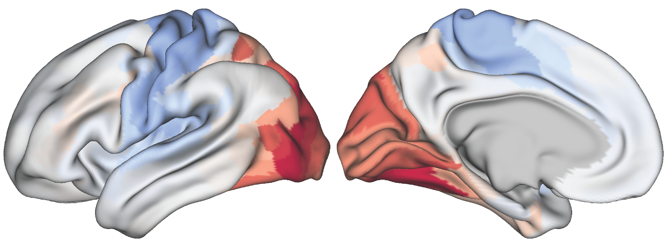
Fig. 2 Parcellated seneorimotor-to-visual gradient map

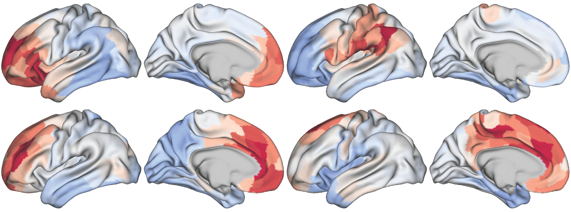
Fig. 3 Randomly permutated seneorimotor-to-visual gradient maps

Note

So far, zoom only supports the automated processing of surface‑based images. For volume‑based images, we recommend using brainsmash to implement the parameterized spatial permutation model, which can be found here.

The single-cell RNA sequencing data

The core functionality of zoom is to compute enrichment scores for SBP‑relevant gene sets at the single‑cell level. To achieve this, we require a human brain single‑cell RNA sequencing (scRNA-seq) dataset. Here, we use the integrated scRNA‑seq dataset of the adult cortex collected by Nano, P. R. et al., which we have re‑integrated and re‑annotated. We then visualize the cell type annotation using scanpy:

>>> import scanpy as sc
>>> adata = sc.read_h5ad("/path/to/integrated.adult_ctx.h5ad")
>>> sc.pl.embedding(
        adata,
        basis='umap',
        color='Cluster',
        title='',
        show=False
    )

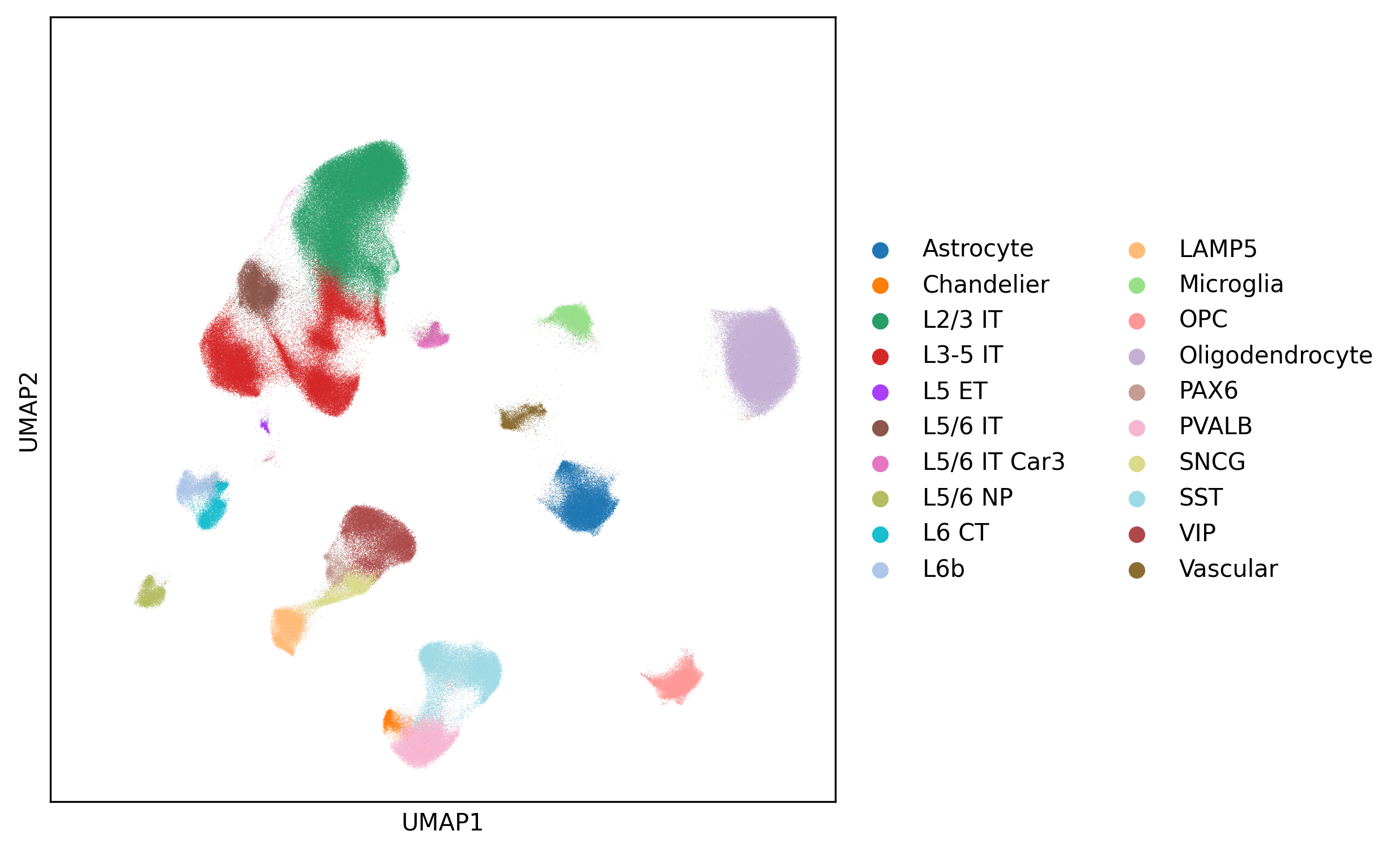
Fig. 4 UMAP plot of scRNA-seq dataset, colored by cell type annotation

Next, to mitigate errors introduced by technical noise and biological replicates in the raw gene expression matrix, while highlighting genes of particular relevance to specific cell subpopulations, we computed the rank‑based Gene Specificity Score (GSS) proposed by Song, L. et al. in gsMap, based on which single‑cell enrichment scores will be calculated. Users can calculate the GSS for scRNA‑seq datasets using the following code:

>>> from zoom import sc_tool as sct
>>> adata = sct.compute_gss(
        adata,
        d=50,
        n_jobs=-1 # use parallel computation
    )

Note

Since zoom.sc_tool.compute_gss() iterates over individual cells, it can be very time‑consuming for large datasets despite parallelization. For reference, processing 500,000 cells on 48 cores takes approximately 12 hours. Please be patient. And we recommend saving the resulting AnnData object from this step to a new .h5ad file.

The above code will add a gss entry to adata.layers. Taking HRH3 as an example, HRH3 is broadly expressed across various cell types in the human cortex. However, the GSS indicates that HRH3 is most critical for a small subset of VIP interneurons, as illustrated below:

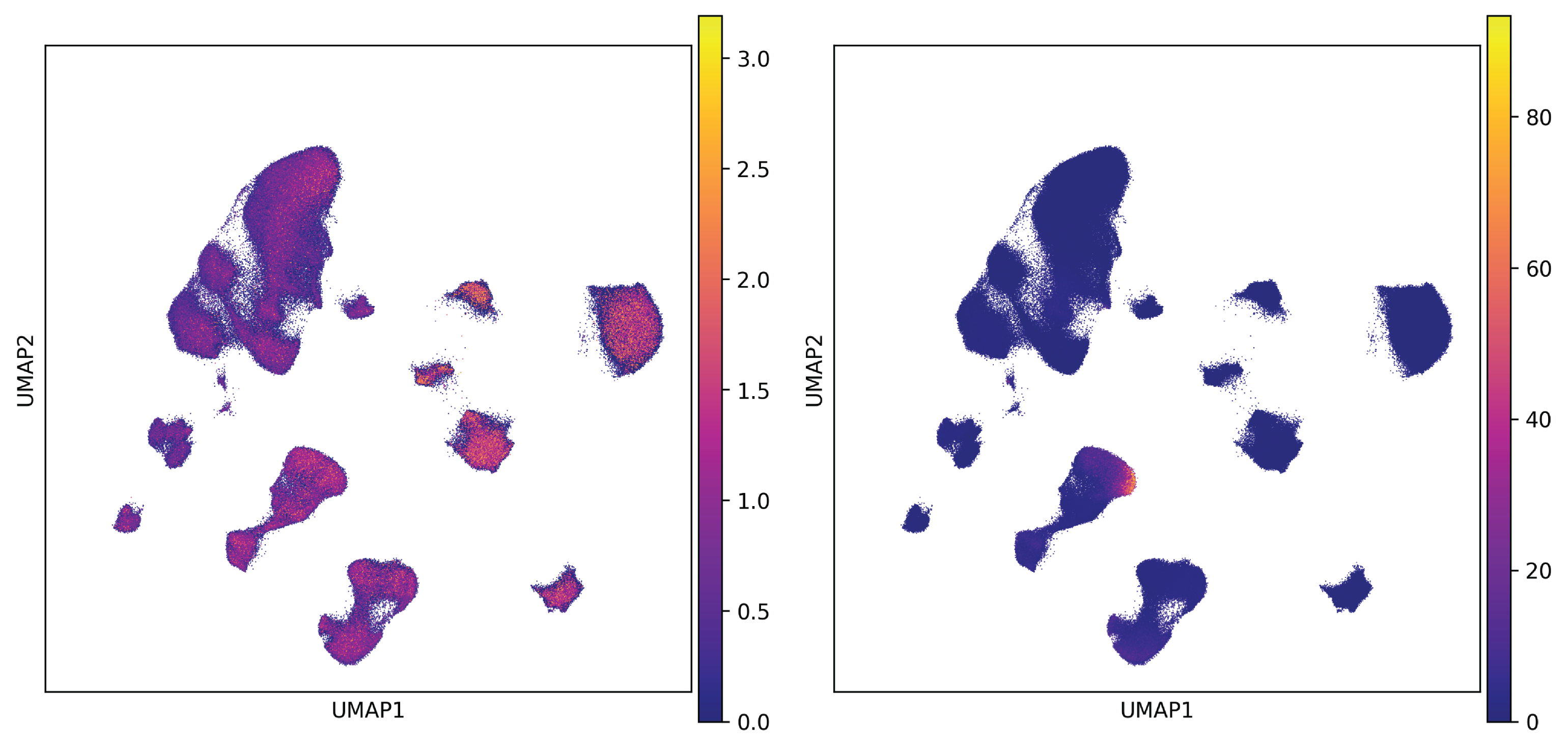
Fig. 5 UMAP plot of normalized expression (left) and GSS (right) of HRH3

Arguments to zoom.sc_tool.compute_gss()

d int, default 50

Number of nearest neighbors for each cell, based on which GSS will be calculated.

gss_limit float, default 200.0

Allowed maximum GSS value to avoid over-representation.

The files produced by the three steps above will serve as inputs to the main class in zoom to associate SBPs with the scRNA‑seq dataset, which will be described in the following sections.